This section contains IHPA’s core concepts and some detailed usages.
If you have no idea of what IHPA is, read the introduction.
If you want to get started to utilize IHPA’s core features quickly, follow the quick start guide.
This is the multi-page printable view of this section. Click here to print.
This section contains IHPA’s core concepts and some detailed usages.
If you have no idea of what IHPA is, read the introduction.
If you want to get started to utilize IHPA’s core features quickly, follow the quick start guide.
Note: Most contents of this page are translated by AI from Chinese. It would be very appreciated if you could help us improve by editing this page (click the corresponding link on the right side).
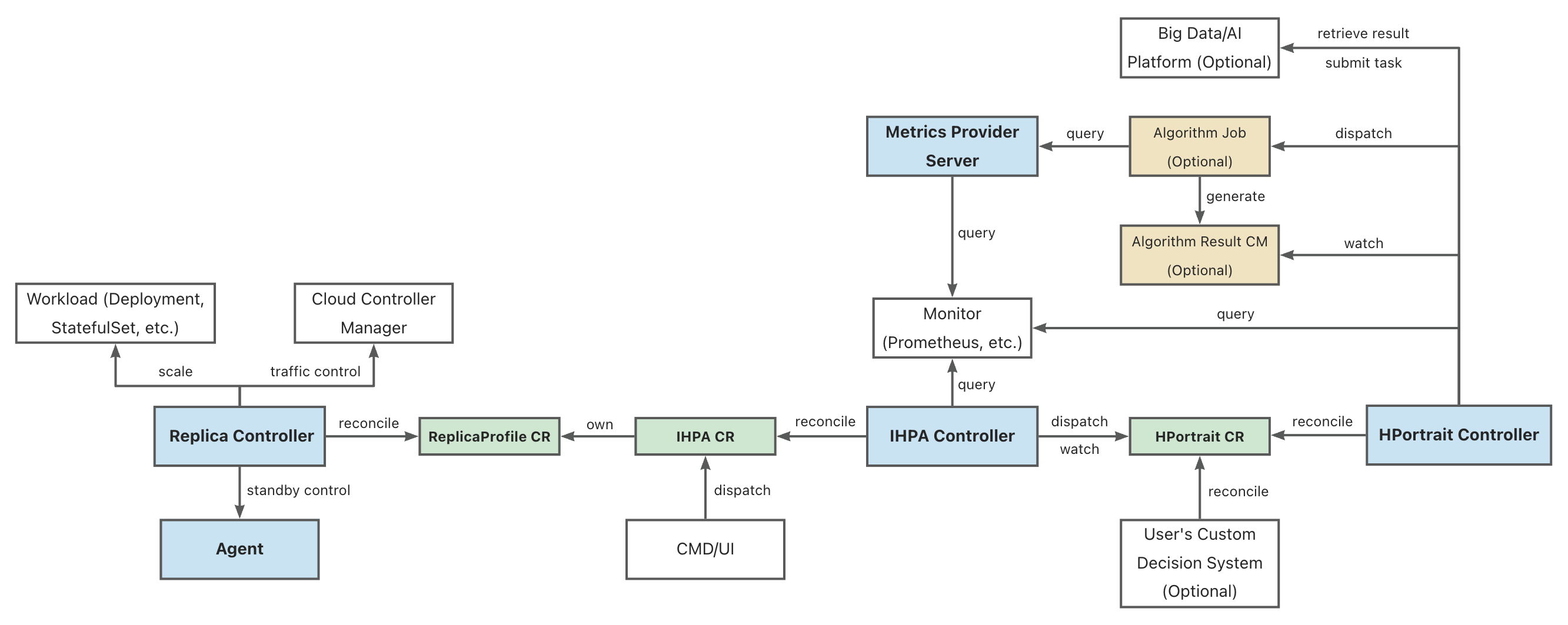
Legend:
Full name of some abbreviations:
Replica Controller is the IHPA execution layer component. It is responsible for the control of the specific workload replica quantity and status. It supports the operations such as scaling, traffic cutoff, and activation of Pods by docking with different native and third-party components.
IHPA Controller is the IHPA control plane component. It directly accepts IHPA configurations from users or external systems (including target workload, metrics, algorithms, change and stability configurations, etc.), issues profiling tasks and integrates profiling results, and then performs multi-level batched elasticity scaling based on the profiling results.
HPortrait Controller is the built-in horizontal elasticity scaling algorithm management component. It is responsible for running and managing the workflows of different elasticity scaling algorithms for different workloads, and converting their output results into standard profiling format. The specific algorithm sub-tasks are scheduled to be executed as separate Kubernetes Jobs or tasks on other big data/algorithm platforms. These sub-tasks obtain historical and real-time metric data from external monitoring systems for computation and generation of profiling results.
Specifically, the logic of some simple algorithms (such as reactive algorithms, etc.) is directly implemented in this component, without going through separate algorithm sub-tasks.
Metrics Provider Server is the unified monitoring metrics query component. It shields the differences of the underlying monitoring system, providing a unified monitoring metrics query service for external running components (such as algorithm tasks, etc.).
The API it provides is similar to Kubernetes Metrics API, but the difference is that it supports both real-time and historical metric queries.
Agent is the agent component running on the nodes of the Kubernetes cluster. It is mainly responsible for executing operations that require interaction with the underlying operating system, such as activating and de-activating Pods.
Note: Most contents of this page are translated by AI from Chinese. It would be very appreciated if you could help us improve by editing this page (click the corresponding link on the right side).
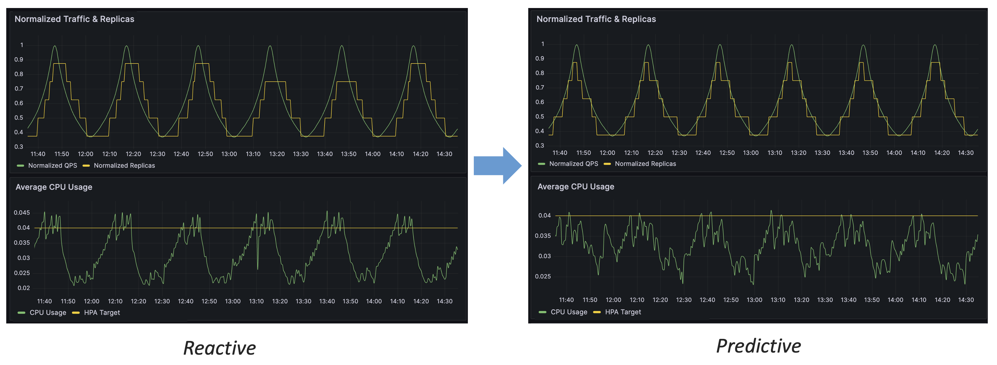
By the comparison of above figure, we can conclude several advantages of predictive scaling over reactive scaling:
In this section, we will introduce in detail the design concept and working principle of IHPA’s “traffic-driven replicas prediction” algorithm.
For online applications, capacity (resource) indicators (such as CPU utilization) are strongly correlated with traffic, i.e., traffic variations drive changes in capacity indicators. Predicting capacity through traffic, rather than directly predicting capacity indicators, has the following advantages:
In order to convert the replica count prediction problem into a traffic prediction problem, we designed a Linear-Residual Model to find the association function between traffic, capacity, and replica count, as shown in the following figure:
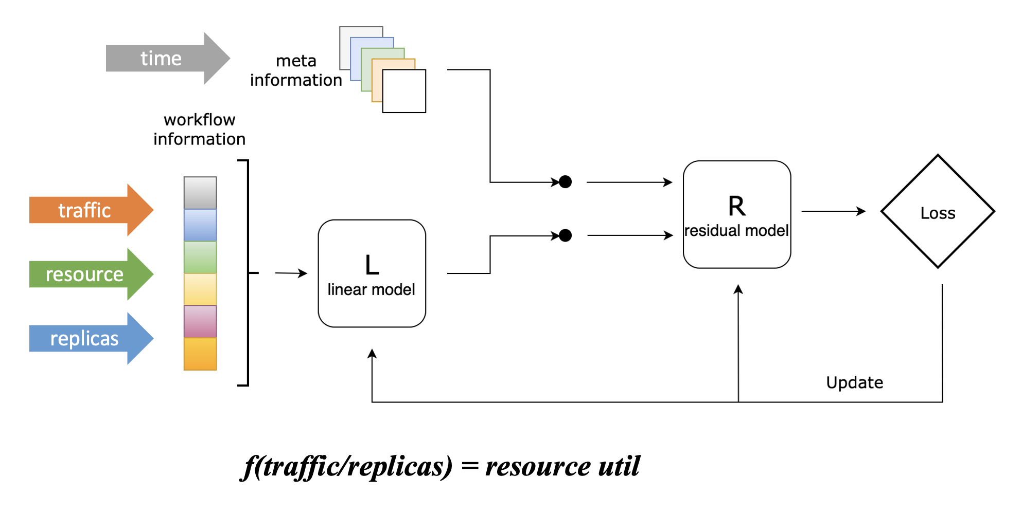
In this model, we set the resource utilization rate as the target indicator, because controlling the resource level of the application is our ultimate goal of using elastic scaling, which is the most intuitive.
However, unlike the reactive scaling algorithm of Kubernetes HPA, although we set the resource utilization rate as the target indicator, this algorithm will not only consider this indicator, but will take historical traffic (supporting multiple lines), historical resource utilization, and historical replica count as inputs. These indicators will first go through a linear model, which can learn the linear association between the three, and get the association function in the above figure; then, they will go through a residual model with other information (currently only includes time information), which will correct the association function after considering other information, and can learn the complex non-linear association between traffic, capacity and replica count.
Here is a simple example to illustrate the main function of the residual model: Suppose an online application executes an internal timed task every Sunday morning, which brings additional CPU resource consumption, but it has no association with the external traffic handled by the application. At this time, this feature cannot be learned through the linear model alone. After introducing the residual model, this model can learn this feature based on time information, so at the time of Sunday morning, we give the same traffic and replica count as other times, and the function it gives will output higher CPU consumption, which is in line with the actual situation.
In the current algorithm implementation, we use ElasticNet as the linear model and LightGBM as the residual model. They are both traditional machine learning algorithms, not strongly dependent on GPU, have lower usage overhead compared to deep learning algorithms, and can also achieve good results. Of course, you can also replace the specific implementation of these models according to your own needs, and you are welcome to provide implementations that you think are superior in certain scenarios.
After using this model to get the association function, we can convert the replica count prediction problem into a traffic prediction problem: knowing the target resource utilization rate, just input the predicted traffic, and you can get the predicted replica count (which can maintain the target average resource utilization rate under the predicted traffic).
Denote workflow information (including traffics, resource usage, replicas) as $k$, target indicator (resource usage) as $y$, and meta information (including time, etc.) as $\omega$. We first use a linear model to characterize the skeleton of target indicator: $$\hat y_l = L(x)$$ Then we calculate the error of the linear model: $$e = y - \hat y$$ Next, we combine meta information with the error of the linear model, and mature it by a residual model: $$\hat e = R(\hat y,\omega)$$ Finally, we get the estimation of $y$ as: $$\hat y_r = \hat y_l + \hat e$$ where $L$ and $R$ could be any linear and residual model.
We designed a deep learning model called Swish Net for Time Series Forecasting to predict traffic indicators over time. This model is specifically optimized for the use case of IHPA and has the following two main characteristics:
| MAE | RMSE | |
|---|---|---|
| DeepAR | 1.734 | 31.315 |
| N-BEATS | 1.851 | 41.681 |
| ours | 1.597 | 28.732 |
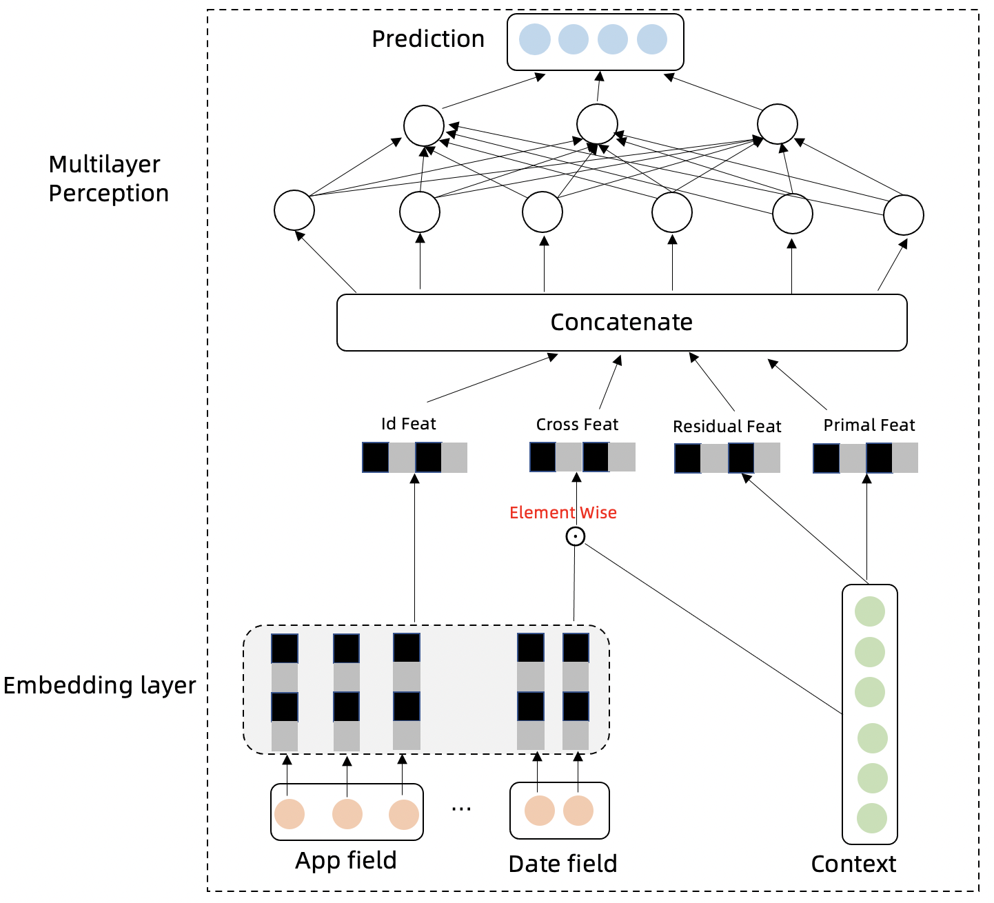
Assuming that the historical traffic $y_{1:T,i}$ is known, the future real traffic is $y_{T+1:T+\tau,i}$, the predicted traffic is $\hat y_{T+1:T+\tau,i}$, and the category of the traffic (such as App) is $i$. The traffic time series will have cyclical, trend, and autoregressive features. We design the following modules to capture these characteristics, and aggregate information to make predictions for the future.
The Embedding Layer of the model projects category information and time information into high-dimensional vectors. The category information expresses the differences between different sequences, and the time information can express the cyclicity of the time series: $$V_i = Embed(i)$$ $$V_t = Embed(t)$$
The cross product of the model’s time and category features with historical traffic can further extract different differential and cyclical features of different sequences: $$\tilde V_i = V_i \odot y_{1:T}$$ $$\tilde V_t = V_t \odot y_{1:T}$$
The difference feature between the next time step and the previous time step of the traffic time series can eliminate the trend and better express the periodicity of the time series. The trend feature is included in the original sequence: $$\tilde y_{1:T} = y_{2:T} - y_{1:T-1}$$
The input and network structure of the Multilayer Perception layer model are expressed as follows: $$in = concate(V_i,V_t,\tilde V_i,\tilde V_t,Embed(i),Embed(t),\tilde y_{1:T},y_{1:T})$$ $$\hat y_{T+1:T+\tau,i} = MLP(in)$$ The multilayer time network summarizes the information of the above feature modules and predicts the time series of future time steps.
The loss function of the model is MSE: $$loss = \sum_{i,t}(y_{i,t}-\hat y_{i,t})^2$$
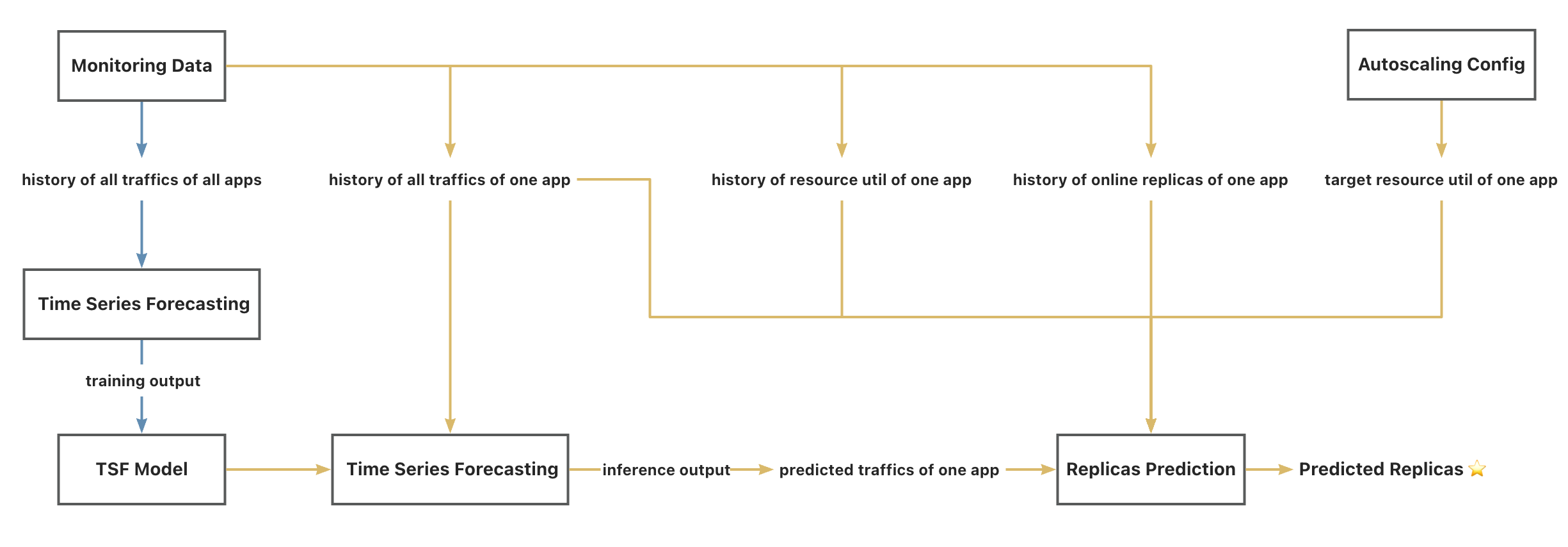
Finally, we can link the above two models with the relevant data sources to get the complete workflow of the IHPA predictive autoscaling algorithm, as shown in the following diagram:
Legend:
Note: